If you’re reading this page, then you might have already heard of the infamous ripple carry adder or even more complex ones like the carry skip adder or select adder. However, there are many interesting ways in which we can add two (maybe even more!) numbers. For those of you that don’t want to look at math too much, you don’t have to look at the delays or the costs (which is where most of the formulas are), but understanding the parallel prefix problem is necessary in order to understand the parallel prefix adders. As usual, the adders will be described in increasing order of complexity, and sometimes build upon principles that were described on previous adders.
A small note before we begin: if applicable, the red path on a diagram represents a critical path. A critical path is defined as a path with greatest delay. Of course, sometimes multiple critical paths are present, but I will only highlight one of them.
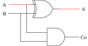
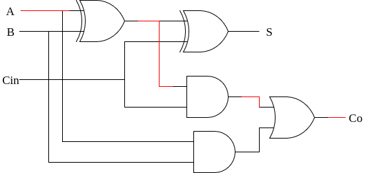
The full adder is the basic building block of, not only the RCA, but also all of the other adders. It mimics the way we do addition on one bit: it adds the carry of the previous block with bits A and B, and produces one bit of result and a carry. The ripple carry adder is made by concatenating several full-adders, and the way it does addition is analogous to the way we do addition by hand. Of course, there are many different ways to formulate a full adder using different logic gates, and some of them are easier to implement at transistor level, but for now let’s forget about transistors. Half-adders are the same as the full-adder, but they don’t take a carry-in. For now let’s forget about them.
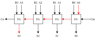
The critical path of the ripple carry adder is the path that goes from \(A_{0}\) to \(S_{n}\).
In order to limit the propagation delay of the ripple carry adder, many other architectures were devised. One of them is the Carry Skip Adder, which aims to reduce the propagation delay by propagating the carries only through a smaller block. But how is that possible? For that, let us analyze how the carry-out relates to the carry-in in function of the 1-bit inputs \(a\) and \(b\).
One thing that you might have noticed is that it’s very simple to check whether a carry propagates through a block of full-adders, we just need to AND all of the \(p\)’s of the block or subsection that you have selected. After all, if even one of the full adders of the block generates or destroys a carry, the carry-out of the block doesn’t depend on the carry-in of the block anymore.
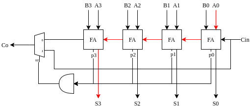
Since we have separated the behavior of the carry-out from the value of the carry-in, we can compute the values of the propagates and carries for each individual block simultaneously. After all, if the carry-in is not propagated, the value of the carry-out will be independent of the value of the carry-in, and due to the structure of the block, if the carry-in is indeed propagated (and the propagates can also be computed in parallel), it doesn’t have to propagate through all of the full-adders and is instead forwarded directly to the next block. There cannot be a critical path with greater delay, since by the time the first carry is computed, all of the (non-propagated) carries are already computed. Therefore the critical path must lie within the propagation path.

With all of that said, there are two important questions that remain: - What is the critical path of the whole adder? - What is the optimal block size? The critical path of the whole adder is the path that goes through all of the full-adders of the first block (generation of the first carry), is propagated through all of the middle blocks and enters the carry-in of the final block and exits through the last bit of the last block. After all, the result is still affected by the carry-in even if the carry-out might not be. For the sake of simplicity, assuming that all blocks are of equal size, and assuming that the time for the generation of the carry-out is equal to that of the generation of the outputs in a full-adder: \[T_{\text{critical}} = 2n_{b}T_{\text{FA}} + (n_{B}-1)T_{\text{MUX}} = 2n_{b}T_{\text{FA}} + \left( \frac{N}{n_{b}} - 1 \right )T_{MUX}\] Where:
With that formula we can already find the optimal number of blocks. We want to find the minimal time of the critical path as a function of the number of blocks, therefore: \(\frac{\partial T_{critical}}{\partial n_{B}} = 0 \implies -2 T_{\text{FA}} + \frac{N}{n_{b}^2} T_{\text{MUX}} = 0 \implies n_{b} = \sqrt{ \frac{NT_{\text{MUX}}}{2T_\text{FA}} } \propto \sqrt{ N }\)
Yes, but this problem is made complex because it also depends on the technology that we are using. This is a solved problem, so if you’re curious you can read more here.
Since we can summarize the propagation of a group of blocks by multiplying the propagation signal of all of their composing blocks, we can add another layer to further summarize the propagate signal of groups of blocks to perform even larger carry skips, making the adder faster.
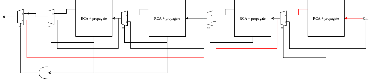
This adder operates on a similar principle to the CSkA, but it has almost double the area, half of the elegance of the CSkA and is a bit more efficient.
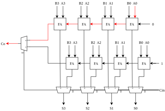
It operates of a very simple principle. It precomputes results in each block for \(C_{\text{in}} = 1\) and for \(C_{\text{in}} = 0\), then it selects a result to be used based on the actual carry-in. For blocks with fixed size, the equation for \(T_{\text{critical}}\) is almost the same as the one for the CSkA (but \(T_{\text{FA}}\) is not multiplied by 2), but it achieves optimal results for variable-sized blocks, specifically if \(T_{\text{FA}} = T_{\text{MUX}}\) (which is unlikely) then the delay is \(\lfloor \sqrt{ N } \rfloor\). Again, if you’re curious, you can read more here.
The carry-skip adders can also be organized into a tree-like architecture, where we use additional multiplexers to give us the carry of the next \(2^k\) blocks to give us a logarithmic dependency on \(T_{\text{MUX}}\).
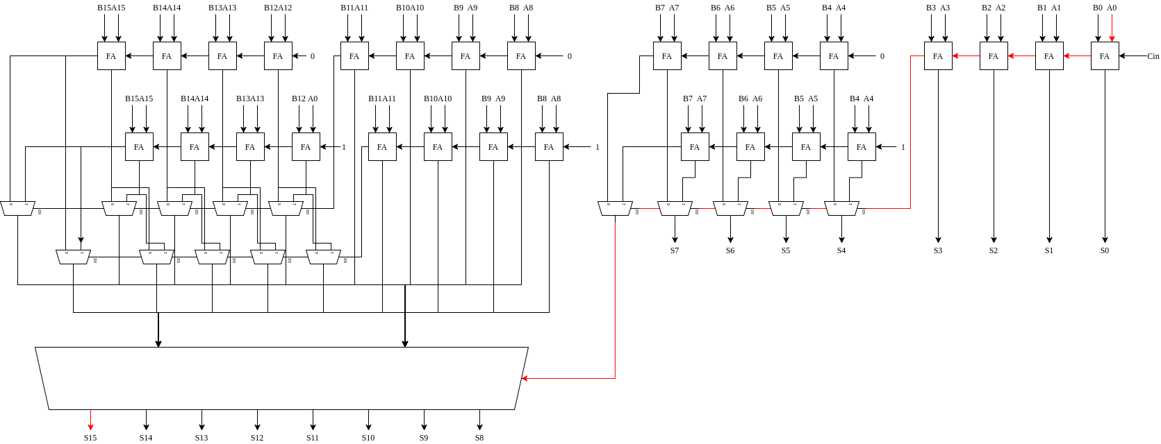
If you haven’t already we recommend you look into this section.
Yeah but it uses principles from the parallel prefix problem. If you understand the parallel prefix problem then you won’t have to hear the simplified explanation for the carry-lookahead adder.
Suppose that we have:
Due to the associative nature of the operator \(+\), we can rearrange the sum to be parallelizable through, for example, divide and conquer strategies. The problem consists in finding the best way to parallelize the sum, which of course can change depending on the problem, and there might be multiple solutions with different trade-offs.
Let us the define:
Small note: Some of you might have realized that the \(*\) operator is idempotent, which really means that \((G_{i:j}, P_{i:j}) = (G_{i:n}, P_{i:n}) * (G_{m:j}, P_{m:j})\) with \(i \geq m \geq n \geq j\), which isn’t terribly useful but interesting.
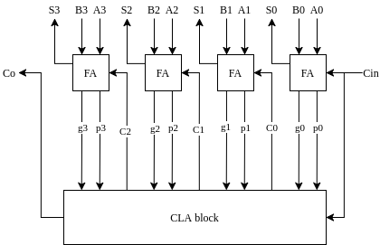
The first of our fast adders. As we already spoiled in the previous section, it is possible to compute whichever carry we want if we have \(C_0\) and the propagate and generate signals for each bit. Of course, we could simply expand the recurrence equations \[c_{1} = g_{0} + p_{0}c_{0}\] \[c_{2} = g_{1} + p_{1} c_{1} = g_{1} + p_{1}g_{0} + p_{1}p_{0}c_{0}\] \[c_{3} = g_{2} + p_{2} c_{2} = g_{2} + p_{2}g_{1} + p_{2}p_{1}c_{1} = g_{2} + p_{2}g_{1} + p_{2}p_{1}g_{0} + p_{2}p_{1}p_{0}c_{0}\] And so on, and implement each carry lookahead block using its full expressions. This way, the carry-lookahead is able to derive its outputs from all inputs that affect it. The carry-lookahead design tries to simplify this ideal, but if implemented this way, it eventually becomes impractical and inefficient. For 4 bits it’s totally acceptable, for 8 bits it’s not, the fan-in (number of inputs) is simply too high.
We can implement the carry-lookahead as a tree. The generate and propagate signals have to be taken all the way to the bottom of the tree, which will then start generating carries and passing them up the tree.
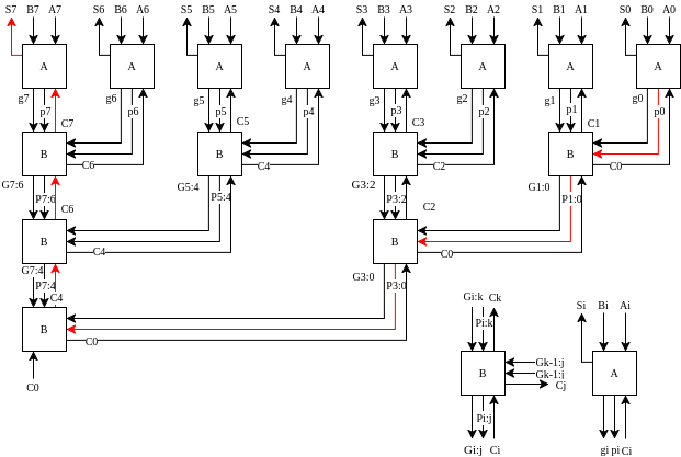
Where:
As you can see, the generate/propagate signals have to be sent down the tree, and only then can the carries be sent up to the adders. Let
Then the delay can be expressed as: \[T_{C} = T_{Af} + T_{Ab} + (\log_{2}k - 1)(T_{Bf}+ T_{Bb})\]
I’ve personally never read anything about it, but it should be possible, I think. With 4-wide B blocks, for 64 bits you only need a tree depth of 2 and the delay becomes \[T_{C} = T_{Af} + T_{Ab} + (\log_{4}k - 1)(T_{Bf}+ T_{Bb})\] Whether it’s worth it or not, I have no idea.
Ah yes, the bread and butter of fast adders. These are structures used in carry-lookahead adders to predict carries and are some of the fastest in town. In this section I will not present all of the parallel prefix networks, only the “classics”. There are many ways we can subdivide addition, and in each one we have to balance the maximum depth (speed), the number of blocks (area) and the fan-out of the network.
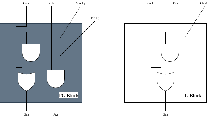
P.S.: From this point until the end of the section, \(k\) refers to the total number of bits.
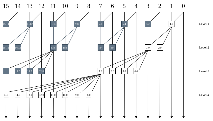
The Ladner-Fischer network utiliizes the classic divide-and-conquer strategy in order to solve the parallel prefix problem. But as you can see the Ladner-Fischer network presents a huge problem: its fan-out is too high! The stage 4 for PG block for bit 7 has a fan-out of 8! And it grows linearly with \(k\)! Because of that it’s not used very often.
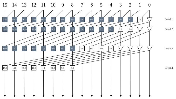
The Kogge-Stone network manages to maintain the same number of stages of the Ladner-Fischer network while solving its fan-out problem, but as you can see, it has a large number of blocks, which means that it has an increased area and power consumption. Still, it is a very fast adder.
They’re buffers. They are used to restore signal strength among other things, but for now you can pretend that they don’t exist.
We have \(log_{2}k\) levels, that’s it’s delay.
As you can see, starting at stage 1, we have \(k - 1\) blocks. At stage 2 we have \(k - 2\) blocks. At stage 3 we have \(k - 4\) blocks, and so on until the last stage where we have \(k - \frac{k}{2}\) blocks. We have \(\log_{2}k\) levels, therefore you can think of the cost as the sum of the area of the rectangle (\(k\log_{2}k\)) minus the area of the missing pieces (\(1 + 2 + 4 + \dots\), it’s a finite geometric series that adds up to \(k - 1\)). In short, \(C(k) = k\log_{2}k - k +1\).
The maximum fan-out is \(\log_{2}k + 1\), which is the fan-out of node 0.
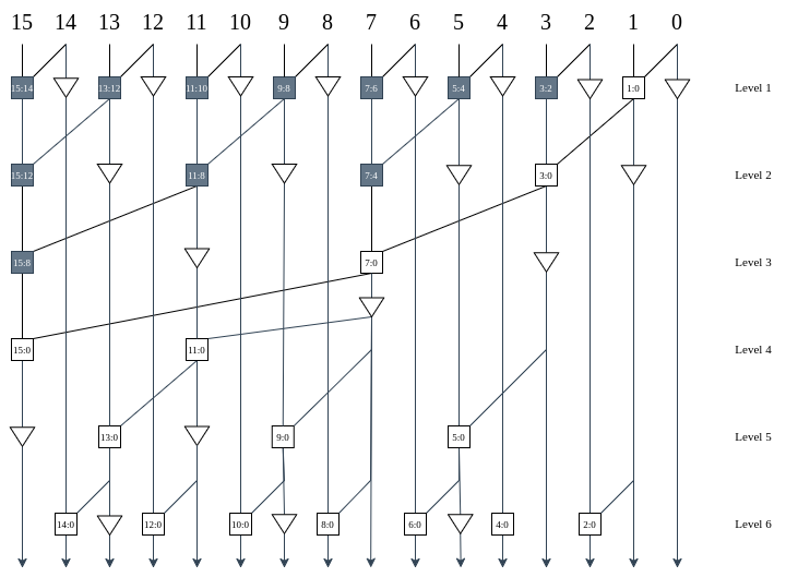
The Brent-Kung network has a bigger delay but it manages to keep the number of wires and the area of the adder reasonable, leading to decreased power consumption.
Notice that the critical path Brent-Kung network is the one that passes through a tree of height \(log_{2}k - 1\) (with root node on row 3 bit 7) and an inverse tree of height \(\log_{2}k - 1\) (with root on row 4 bit 11), therefore the total delay is going to be \(2log_{2}k - 2\). If you want the recurrence equations related to the recursive construction of the Brent-Kung network, I myself admittedly don’t understand them quite well, but you can have them: \(D(k) = D(k/2) + 2 = D(k/2^h) + 2h\), with \(k/2^h=2\) and \(D(2) = 1\) we have \(h = log_{2}k - 1\) and \(D(k) = 2\log_{2}k-1\) which is really \(2\log_{2}k - 2\) for reasons unknown to me.
Again, using the tree intuition, let us instead visualize the full trees. The adder is composed of a one tree with root node on bit 15 and another tree which should have root on bit 0. But all of the nodes on bit 0 were removed. Therefore we have \(2(k - 1) - \log_{2}k\) nodes. Again, if you want the recurrence equation: \(C(k) = C(k / 2) + k - 1 = 2k - 2 - \log_{2}k\)
I hope you liked your journey up until this point, you can now take a breather. Even if there are more complex optimization techniques for adders and CLA networks, such as using high-radix adders, or mix and mashing different adders, I’d like to think that I’ve imparted all of the basics unto you. If you come across one of those in the wild, you at least have the basis necessary to face it.
Ok, hear me out. There is one more thing I have to introduce to you, which is going to be fundamental for the next topic: multipliers. But this is not hard. Have you posed yourself the question:
Yeah, we can concatenate more adders. But what if we want to add, for example, 32 numbers? Do we really need 32 adders? Do we need to turn the adder into a sequential circuit?
You might have noticed something: The full-adder does not add 2 numbers. It adds 3 numbers. More specifically, it adds 3 single-digit numbers and produces a single double-digit number. In a more formal terminology, it acts as a 3-2 compressor. Let us suppose that you want to add 3 numbers You can, therefore, use N full-adders to reduce these 3 numbers to 2 numbers and then you can use a normal adder.
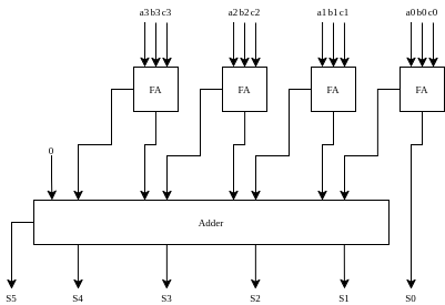
Of course, this extends nicely even if you have more numbers, which is going to be the basis of CSA multipliers.
As you might know, if we are using two’s complement, \(a - b = a + \bar{b} + 1\). With this knowledge, we don’t need to have a dedicated subtractor. We can handle the negation, but how do we handle the \(+ 1\)? It’s very simple actually. We just have to pass it through the carry-in of the adder. If we are to build an ALU, we just need a control signal which is XORed with all bits of b (so we have \(\bar{b}\) when \(\text{sub} = 1\), otherwise \(b\)) and enters the carry-in of the adder (so we have \(\bar{b} + 1\) when \(\text{sub} = 1\), otherwise \(b\)).